ROOTSNNS: a ROOT interface to SNNS
Manual and Examples

• What is ROOTSNNS?
• Installation
  • System requirements
  • Getting the code
  • Compiling from source
• Using ROOTSNNS
  • Preparing the data
  • Creating neural network
  • Neural network initialization
  • Training neural network
  • ROOTSNNS output files
• Plotting and Analyzing Tools
• Examples
• Known Problems
• Authors

Download ROOTSNNS

Classes and members API reference

Development page

What is ROOTSNNS?

ROOTSNNS is a collection of C++ classes providing a flexible environment in which one can easily build, train, and test multiple neural networks (NN). The core NN functionality is supplied by the Kernel User Interface libraries of the Stuttgart Neural Network Simulator (SNNS). SNNS is a self-contained tool with a numerous handy utilities and plenty of options for the control of the NN training. With all its excelence SNNS provides only one, though generic, way of sucking in the inputs and spitting out the results, that is by means of ordinary text files. However, in some studies the number of training samples can be very large and an optimal input configuration is not known a priori. Having this in mind the authors of ROOTSNNS realized that using text files is not feasible when additional analysis is required on either or both input and output data. ROOT, a data analysis framework, seems to be an excelent choice for that task. In ROOTSNNS the input and output data, along with NN performance, can be retrieved from or saved into ROOT TTrees while supplementary results can be saved in histograms.

One can use ROOTSNNS to call SNNS methods directly from ROOT interactive environment (CINT) or from user's own stand-alone C++ program. Alternatively, ROOTSNNS provides a number of convinience methods for training a NN and data management.

If one wants to "just use a NN", the combination of ROOT, SNNS and the described interface might be the answer. The setup is quick and there is virtually no learning curve. Moreover, both SNNS and ROOT can be obtained by anyone for free, so is ROOTSNNS, by the way.

Installation

System requirements

In order to get going one needs a computing platform that ROOT and SNNS can work on (this potentially includes even some versions of MS Windows). In practice, however, the setup has only been tested to work on a somewhat limited subset of such computing platforms, that is to say a Linux machine with ROOT installation is implied in what follows.

Normally, 50 MB of user disk space should be enough for ROOTSNNS installation: 38 MB for SNNS installation, including binaries, and 12 MB for ROOTSNNS installation, most of which is taken by the complete example. Superuser privileges are not needed, so user's home directory should be a perfect place to install to.

Getting the code

The ROOTSNNS code can be downloaded from the project's download page. It is recommended to download the latest stable release of the code.

One can also get the latest (not neccesarily working) code from the CVS repository by executing the following command

  cvs -z3 -d:pserver:anonymous@cvs.sourceforge.net:/cvsroot/rootsnns co -P rootsnns

Compiling from source

The ROOTSNNS classes are compiled into a single shared object library. It is up to the user to decide whether to link this library against a standalone program or load it into an interactive ROOT session. We provide examples for both cases.

As a first step, a few environment variables need to be set. ROOTSYS and SNNS_DIR must point to the directories where you have ROOT and SNNS installed. In (t)csh shell the following should do the job:

  $>setenv SNNS_DIR path-to-SNNS-dir
  $>setenv ROOTSYS  path-to-ROOT-dir

Next, make sure that the following directories are added to the list of searchable paths for executables:

  $>setenv PATH $ROOTSYS/bin:{$PATH}
  $>setenv PATH $SNNS_DIR/tools/bin/i686-pc-linux-gnu:{$PATH}

Finally, add the path where ROOT shared libraries reside to the runtime environment variable:

  $>setenv LD_LIBRARY_PATH $ROOTSYS/lib:{$LD_LIBRARY_PATH}

At this point the ROOTSNNS shared object library can be compiled with the help of make utility by simply executing

  $>make lib

It is not unusual to have long jobs when training a neural network. In such cases it can be more convenient to run a batch job as stand-alone executable. It is advisable to compile and run an example which is included in the distribution. This can be done by executing

  $>make main-train
  $>./main-train

Using ROOTSNNS

Preparing the data

Next, prepare two ROOT files, for definitiveness we will call them train-sig.root and train-bkg.root, to be used in NN training. Each should contain a TTree of patterns. The important thing is that the structure of the tree (the name of the tree, number/names of branches/leaves) is the same between the two files and matches that of the tree you get by running on the actual data (which you want to apply the NN function to). The train-sig.root and train-bkg.root included with the ROOTSNNS distribution are used in the example, which you may want to play with before you start your own project. The details of the example are described in this section. In the following we assume that the name of the tree of patterns is all.

Start a ROOT session and execute the following macro:

  .x macros/makeNNVars.C("train-sig.root", "all")

Creating Neural Network

Initialization of Neural Network

Training Neural Network

ROOTSNNS output files

Take a look at the results directory (results). It should look something like this:

  drwxr-sr-x  3 jbond  cdf     4096 Dec  2 11:20 ./
  drwxr-sr-x  9 jbond  cdf     4096 Dec  2 11:20 ../
  drwxr-sr-x  2 jbond  cdf     4096 Dec  2 11:20 CVS/
  -rw-r--r--  1 jbond  cdf     1791 Dec  2 17:50 n_2_2_1_v0v1.net
  -rw-r--r--  1 jbond  cdf  6958698 Dec  2 17:52 out-train.root
  -rw-r--r--  1 jbond  cdf     2799 Dec  2 17:54 v2n2.C    

  -rw-r--r--  1 jbond  cdf     1784 Dec  2 17:43 tmp-ep00050.net
  -rw-r--r--  1 jbond  cdf     1784 Dec  2 17:44 tmp-ep00100.net
  -rw-r--r--  1 jbond  cdf     1784 Dec  2 17:45 tmp-ep00150.net
  -rw-r--r--  1 jbond  cdf     1784 Dec  2 17:46 tmp-ep00200.net
  -rw-r--r--  1 jbond  cdf     1784 Dec  2 17:47 tmp-ep00250.net
  -rw-r--r--  1 jbond  cdf     1784 Dec  2 17:48 tmp-ep00300.net
  -rw-r--r--  1 jbond  cdf     1784 Dec  2 17:49 tmp-ep00350.net
  -rw-r--r--  1 jbond  cdf     1784 Dec  2 17:50 tmp-ep00400.net
  -rw-r--r--  1 jbond  cdf     1784 Dec  2 17:51 tmp-ep00450.net
  -rw-r--r--  1 jbond  cdf     1784 Dec  2 17:52 tmp-ep00500.net

Now open file out-train.root in ROOT's TBrowser. You should see two trees (PATTERNS and PERFORMANCE) and two histograms (histTrainError\_nn\_name and histValidError\_nn\_name). The PATTERNS tree (branch vars) contains all the input patterns which are supplemented by at least two additional fields:

• type (typically takes on one value from \{"train", "valid", "test"\})
• target0

There can, in principle, be more than one target (then you should expect to find target0, target1, etc.), e.g., training to distinguish b jet from non-b jet and quark jet from anti-quark jet at the same time would require two targets. All the other variables are listed as var00, var01, var02, etc. This is done to avoid names like "(vars.X+vars.Y)/2" which one would have to deal with if the names of the input variables are particularly complicated. var00, var01, var02, ... correspond to the input variables arranged in alphabetic order.

The PERFORMANCE tree should only be interesting if you trained more than one NN in the same job, e.g., you wanted to see which number of hidden nodes in the range from 5 to 15 allows the most efficient use of information, i.e., it is only of interest if you would like to compare different NNs. histTrainError\_nn\_name histogram shows the NN generalization error vs. epoch number on the training sample. This should generally be a falling distribution (not without occasional fluctuations). histValidError\_nn\_name shows the generalization error calculated on the validation sample as a function of epoch number. It should also exhibit decreasing behavior, at least until a certain number of epochs beyond which the NN gets seriously over-trained. The epoch at which this histogram has a minimum is the one for which optimal NN is saved.

The following will create a ROOT(C++) function based on the saved NN (n\_2\_2\_1\_v0v1.net file):

  cd results
  $SNNS_DIR/tools/sources/snns2root n_2_2_1_v0v1.net v2n2.C

Upon successful execution, the above will produce v2n2.C file which contains the definition of the NN function snns(float* pattern, float*, output). This function can be called from ROOT, e.g., after .L v2n2.C+.

Go back to the main directory (cd .. if you are in the results), start a ROOT session and do

  .x macros/check.C

This should generate a canvas which shows NN output distribution for signal and background as well as the ``Purity vs. NN output'' plot. It also calculates the generalization error for the trained NN. The check.C macro would only work if you had designated part of your training sample for testing. It should work ``out of the box'' on the example results/out-train.root that comes with fresh ROOTSNNS, but only trivial modifications are needed in order to make it work for your specific NN.

Examples

ROOTSNNS distribution includes an example to demonstrate typical use of the interface. The step by step instructions described in sections above have been executed for this example. In particular, the NN has already been trained using 30K+30K patterns for training and 30K+30K patterns for validation (signal+background). One can verify this by browsing results/out-train.root. If you want to train the NN yourself (maybe to play with some training settings), all you need to do is to execute the following commands:

  setenv SNNS_DIR path-to-SNNS-dir
  setenv PATH $SNNS_DIR/tools/bin/i686-pc-linux-gnu:{$PATH}
  gmake
  ./main-train.exe

The example deals with a rather common situation in which one observes a peak on top of a slowly varying background in the mass (M) distribution. Both signal and background are characterized by two other (correlated) properties X and Y as shown in Fig. 1. One wishes to improve S/(S+B)$^{1/2}$ by some elaborate selection involving variables X and Y.

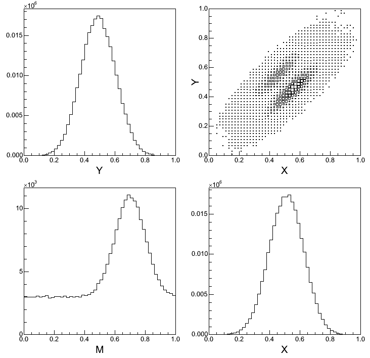
Fig. 1: M, X, and Y, as well as Y vs. X distributions from (pseudo)-data.

The X and Y distributions of signal and background are known (say, from Monte Carlo and data mass sideband respectively) as shown in Fig. 2.

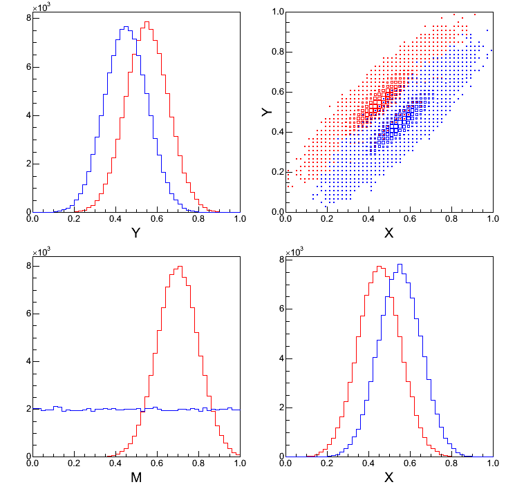
Fig. 2: M, X, and Y, as well as Y vs. X distributions separately for signal (red) and background (blue).

Unfortunately, background X distribution is quite similar to that of the signal, so any direct cut on variable X is going to either cut out too much signal or not improve peak significance enough. The situation with a direct cut on variable Y is much the same. Leaving out such techniques as Fisher discriminant and likelihood ratio (which would actually be quite appropriate in this simple case of only two variables/properties), one wishes to train a NN to achieve as much signal/background separation as possible.

A training has been done using train-sig.root and train-bkg.root that come with the ROOTSNNS distribution. The structure of the TTree in each of these two files, as well as in the data.root file, which the trained NN is going to be applied to, is shown in Fig. 3.

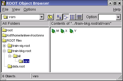
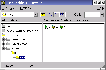
Fig. 3: TTree structure found in train-sig.root~(top), train-bkg.root~(middle) and data.root~(bottom). The tree name is all, and the branch vars has three leaves M, X, and Y (the distributions of M, X, and Y, as well as Y~vs.~X are shown in Fig. 2 for train-sig.root in red and train-bkg.root in blue).

The trained NN has already been exported into results/v2n2.C file, so one can now run macros/check.C script to take a look at the NN distributions for signal and background as well as the ``Purity vs. NN output'' plot. These are shown in Fig. 4.

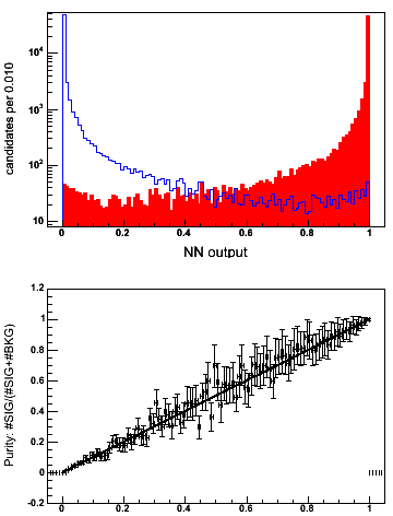
Fig 4: Top: NN output for signal (solid red) and background (blue contour). Bottom: Purity vs. NN output distribution, which should be linear for the optimally trained NN (if the number of signal and background events used to make the plot is the same). The line Purity~=~NN~output is overlaid to guide the eye.

At this point you may also wish to do (having started a fresh ROOT session)

  .x macros/optim.C

Fig. 5: Efficiency vs. Purity plot. Blue (downward looking) triangles represent a scan over the grid of rectangular cuts. Red (upward looking)triangles represent variation of the NN~output cut in the range from 0.5 to 0.95. In a very large range of values NN~output cut keeps almost all of the signal (efficiency near 1) and rejects almost all of the background (purity near 1). No combination of rectangular cuts approaches that.

Figure 6 shows M distribution for the rectangular cuts (left) and NN output cut (right) that result in the best S/(S+B)$^{1/2}$ out of all other (combinations of) cuts in the respective category.

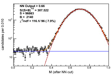
Fig. 6: Fits to (pseudo-)data at the optimal values of rectangular cuts (left) and at the optimal NN output cut. With the optimal NN output cut S/(S+B)$^{1/2}$ of 308 is about 46\% better than 210 achieved with the optimal rectangular cuts. With rectangular cuts S/(S+B)$^{1/2}$ of 308 can only be achieved if the statistics of the (pseudo-)dataset is roughly doubled!

Known Problems

In this section we list known problems which we encountered at various stages of the development.

• There is a known conflict between SNNS and ROOT.

     $g++ -O -Wall -fPIC -Wno-deprecated -pthread
     -I/d0usr/products/root/Linux-2-4/v4_04_02b_fbits_eh-GCC_3_4_3-opt/include
     -c rootsnns_dict.cxx
     In file included from
     /d0usr/products/root/Linux-2-4/v4_04_02b_fbits_eh-GCC_3_4_3-opt/include/Api.h:68,
     from
     /d0usr/products/root/Linux-2-4/v4_04_02b_fbits_eh-GCC_3_4_3-opt/include/RtypesImp.h:19,
     from rootsnns_dict.cxx:27:
     /d0usr/products/root/Linux-2-4/v4_04_02b_fbits_eh-GCC_3_4_3-opt/include/DataMbr.h:63:
     error: expected identifier before numeric constant
     

  The former defines a constant UNKNOWN in snns_glob_typ.h file, while the latter defines UNKNOWN as a global enum type in $ROOTSYS/include/DataMbr.h. The conflict is resolved by adding prefix UNIT_ to constants in snns_glob_typ.h.

Authors

Questions and comments can be sent to the authors of ROOTSNNS:

Konstantin Anikeev <cyberkost at users.sourceforge.net>

Dmitri Smirnov <dsmirnov@fnal.gov>